Artificial intelligence is a vague term for computer applications that carry out some kind of decision making. In general, we’re more inclined to call something AI the more sophisticated and independent its decision making capabilities are. AI are usually designed for a single task or a small collection of related tasks. Many tasks we would like AI to do are simply too computationally difficult. In recent decades, however, increases in available computing power and breakthroughs in AI design have made AI much more versatile and proficient.

Now, with AI at the center of much media frenzy, you may be curious about how they work, what technological developments have been driving progress in AI research, and what kinds of limitations these systems have. My goal is to explain these ideas at a high level while providing simple examples that illustrate the mechanisms of AI.

Note: this is a simplified explanation, and there is nuance that is glossed over.

AI brains: neural networks

Most of the recent development in AI research has been focused on AI that use neural networks (“neural nets”) along with machine learning algorithms. Bear in mind that not all AI uses this technology, and not all applications that use this technology are AI in the traditional sense.

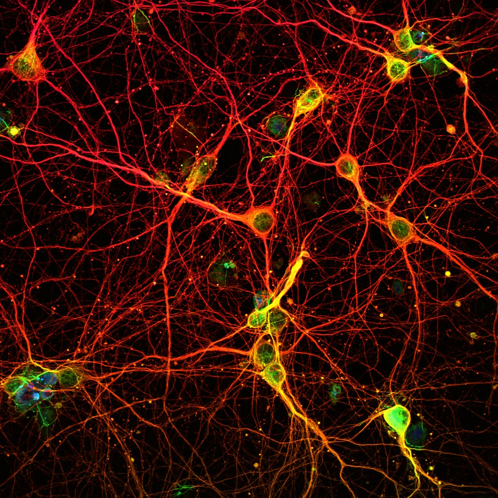
In human brains, neuron cells are chained together into complex networks. Information can only pass through a neuron in one direction: the electrical impulse starts in the dendrites and travels the length of the cell to the axon, where it can jump the synapse to activate adjacent neurons. These impulses originate from chemical reactions in the brain, which create voltage by chemically breaking molecules into electrically charged ions. Depending on the impulse, it may eventually reach muscle tissue, where another chemical reaction will cause the muscle tissue to contract, moving a part of the body.

Computer neural nets are named as such in analogy to human brains. Information (in the form of binary data, or “bits”) is passed from one “neuron” to another through a complex network. Information typically only travels one way, as in biological neurons. At the end of the process we get some binary data output, which might get interpreted as something like text or an image.

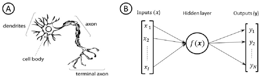
In the intermediate steps, where information is passing from neuron to neuron, what happens is defined not only by the structure of the network (how many neurons there are and how they are connected) but also how individual neurons modify the signal. In biological neurons, this is an electrochemical signal. In neural nets, the signal is numerical and individual neurons apply mathematical functions to those numbers.

Notice in the diagram above that the input to the neural network is actually a list of inputs, and the output is a list of outputs. This has to do with how we conceptualize and organize the information we’re giving to or receiving from the AI. We want the input to the AI to be something meaningful, like a text prompt for a chatbot. In order for the neural net to “understand” the thing we’re trying to show it, we must break it down into constituent parts or properties. For example, suppose we want an AI that will predict the value of a car. We can’t input the car itself into our computer, so we need a way of “digitizing” it. We might describe the car digitally for the AI as follows:

[ manufacturer, model, year, mileage, color ]

We would want more detailed information in real life, but for this example we’ll use these five properties to try to determine the car’s value. Despite the fact that only three of the five are numerical, they can all be represented numerically. For example, we can arbitrarily assign red to 0, blue to 1, white to 2, and so on. As long as we’re consistent, it doesn’t matter what the specific numbers are. All this means that what we really have for input, regardless of what real-world thing we’re talking about, is a list of numbers. This is a vector in math or usually known as an array in computer science.

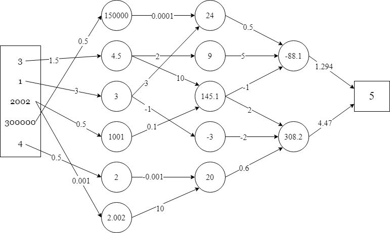
Suppose we have a silver 2002 Honda Civic with 300,000 miles, which we’ll represent as the vector:

[ 3, 1, 2002, 300000, 4 ]

The neural net is arranged in layers. Each input number is connected to neurons in a specific way with weighted connections. Multiple incoming values get added together. This is called a linear combination.

A linear combination of values x₁, x₂, …, x_n is the sum a₁x₁ + a₂x₂ + … + a_nx_n where the a_i are real numbers.

For example, the value of -88.1 below comes from the linear combination:

0.5(24) + 5(9) + -1(145.1)

Where 24, 9, and 145.1 are the incoming values and 0.5, 5, and -1 are their respective weights. (This is similar to the idea of a weighted average.)

This is how the neural net processes data, and this is why an AI’s “thought process” can’t be understood in terms of an ordinary algorithm. The number 4.5 in the first layer below doesn’t represent any meaningful quantity, it’s just an intermediate calculation before the final answer is reached. The output can be interpreted meaningfully: apparently, our car is worth $5.

So the numbers represent something at the beginning, when we input them, and they represent something at the end, when we get the output, but they don’t really represent anything in the middle, where the neural net is doing its work. These layers are referred to as hidden layers because they are treated as a “black box.” What’s happening in the hidden layers is successive calculations of linear combinations.

Tensors and nonlinearity

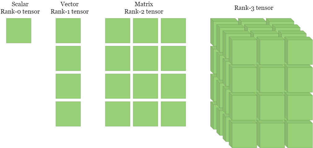
Some background: an ordinary (real) number is sometimes called a scalar. As we have seen, an ordered list of scalars is a vector. A 2D version, a rectangular table of scalars (or an ordered list of column vectors) is a matrix. In fact, each of these concepts is progressively more general: a scalar is both a vector with one element and a 1×1 matrix, and a vector is a columnar matrix. All of these are examples of tensors, the general concept of an n-dimensional array of scalars. The dimension of a tensor is technically called its rank.

I buried the lead by describing the input to a neural net as a vector above and giving an example where that was the case. The input is actually a tensor. The hidden neurons still operate the same way, making linear combinations of scalar values pulled from the input (or from lower layers).

Actually, there is a complication to what the neurons do. So far the math we have described is all linear algebra, which makes computations convenient but has fundamental limitations. The key to neural nets’ computational power is the introduction of nonlinearity through the strategic use of nonlinear functions.

Recall that a linear function is something like y = 3x + 5.

Nonlinear functions are everything else. This includes roots, exponents, trigonometry, calculus, factorials, logarithms, and so on.

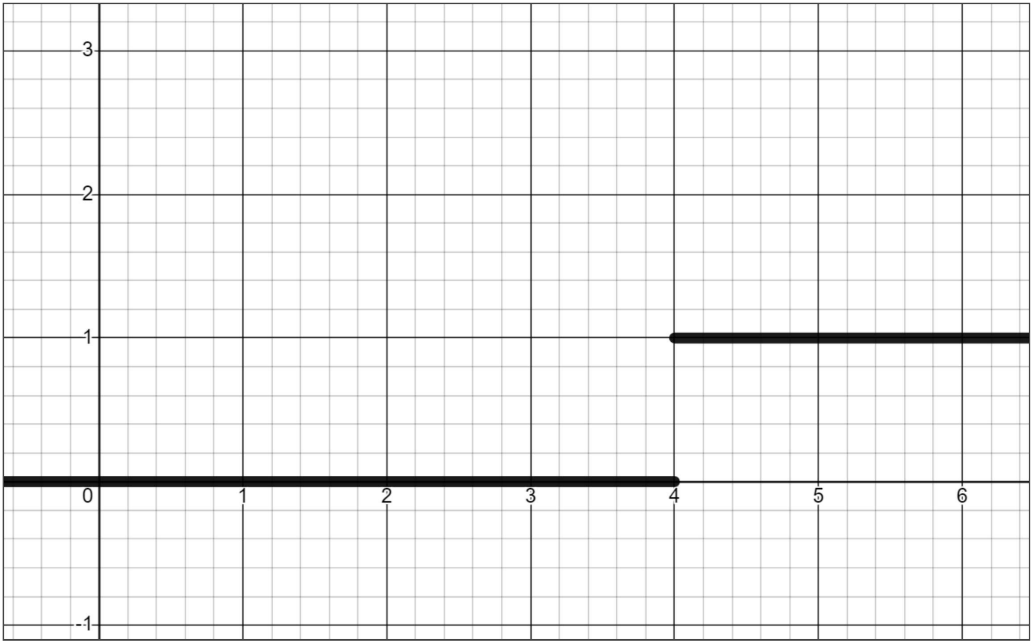
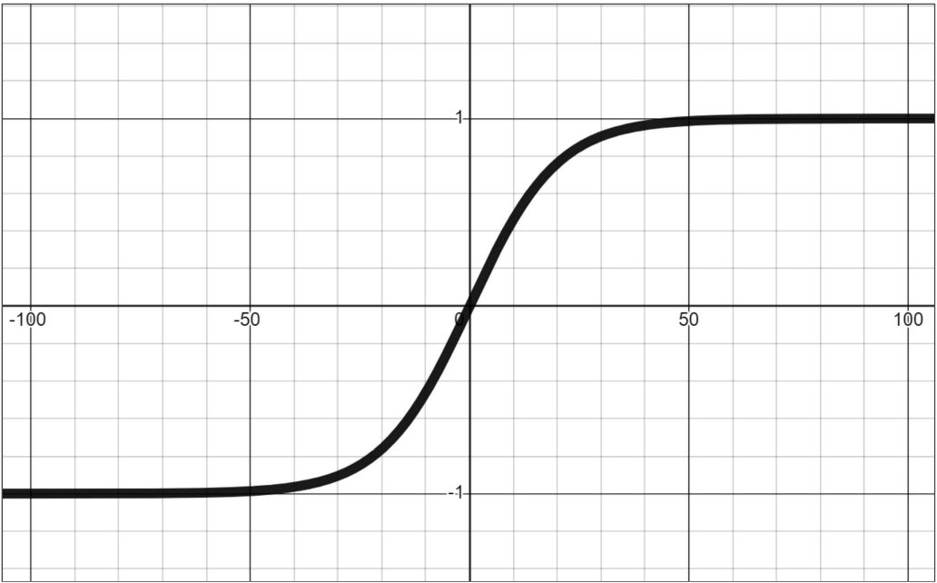
An example of why we might want to use a nonlinear function in a neural net is to introduce a threshold for transmitting or blocking a signal. For example, a function could return 0 if the input is below the critical value and 1 if the input is above the critical value. Nonlinearity can also be used to normalize a wide range of values into values between -1 and 1 (or some other bounds).

Additionally, although I stated above that information typically only travels in one direction, there are exceptions. In some neural net designs, information can propagate backwards.

Machine learning

Neural nets’ hidden layers are created not by programmers setting individual values by hand, but rather by a process of training. The network must be set up initially before training can begin, but the process of making it do a specific task happens through training. There are a few different ways AI can learn. Learning by example involves being provided inputs and outputs and adjusting the network weights to accommodate them. In learning by reinforcement on the other hand, the AI needs a way of determining if its output is good or bad. This strategy involves some trial and error, adjusting weights in the network and evaluating whether the changes make the output better or worse. These are not the only ways of training AI, but they are two of the major ones. A machine learning algorithm may combine multiple learning techniques, and each algorithm is tailored for the data that that particular neural net will be working with.

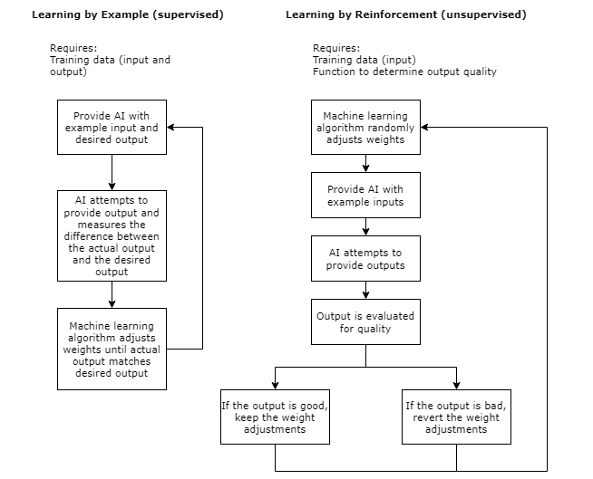
Learning by reinforcement can be useful when there is no single, best output that is known to the programmer in advance.

AI are only ever as good as their training data. This can cause problems since training data is often biased. For example, when teaching an AI what humans look like, we might gather some photos randomly from the internet to use for training data. Even if this data set is representative of photos of humans (which is somewhat doubtful), not all humans are photographed at the same rate. Residents of wealthy countries are much more likely to have their photo appear online than residents of poor countries on average. There could additionally be factors like culture that affect rates at which people appear in photos, for example it might be the case that more American women have photos online than American men. This type of bias is difficult to avoid, especially in cases where we aren’t sure exactly what biases are present (which is most of the time). As a result, AI has a general tendency to unintentionally reproduce or reinforce status quo norms and power structures.

GPUs and computational complexity

Let’s discuss 3D computer graphics for a moment. In something like a 3D animated video, the 3D virtual objects have already been rendered into images, and your computer only needs to display the images on the screen. In a video game, on the other hand, your computer must render the 3D environment into an image before displaying it on the screen. Asking your computer to render frames many times per second while also running all the other aspects of the game is extremely computationally intensive, which was a major limitation for game developers. The reason why early 3D games consisted of simple polygons is because of hardware limitations.

In 1999, Nvidia released the first ever consumer graphics processor unit (GPU) or “graphics card.” The purpose of the GPU is to handle the calculations for rendering 3D graphics, freeing up the CPU to work on other things. Since a CPU is general-purpose while a GPU is specialized, a GPU’s physical processor hardware is optimized for performing very specific types of calculations: namely, those needed to render 3D graphics. In other words, a GPU is not simply extra processing power, it’s processing power for a specific task.

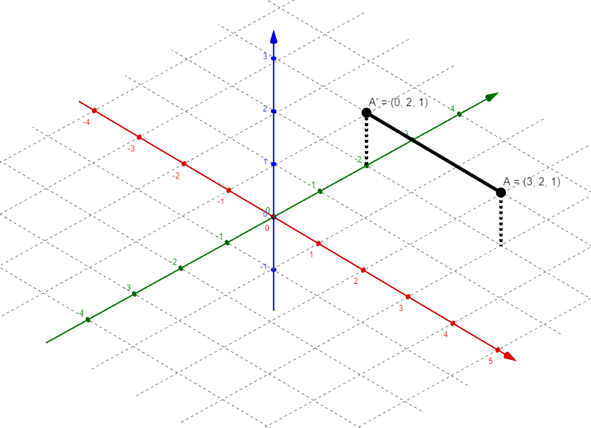
So what computations does a GPU do, you may ask? I will give a typical example. One task in rendering 3D graphics is projecting the 3-dimensional environment onto the 2-dimensional screen. Let’s consider a point in the 3D space and try to figure out where that point will be located when projected by a simple projection.

The point A in 3D space has coordinates (3, 2, 1). We can alternatively interpret these coordinates as a vector, [3, 2, 1]. This is helpful because it enables us to use matrix multiplication. If we want to project point A onto the y-z plane, then we have the projection matrix, P, and the matrix equation PA = A’.

---

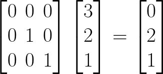
In general, it turns out that much of graphics rendering (including raytracing or “RTX,” shading, perspective, and so on) are linear algebra (matrix) problems. Long story short, the video game industry inadvertently created a situation in which many people have a specialized linear algebra processor in their computer. The general usefulness of GPUs for this kind of computation is perhaps most obvious in cryptocoin mining, which notoriously drove up demand for GPUs beyond what manufacturers had anticipated and inflated GPU prices.

One of the primary differences between CPUs and GPUs is in the number of constituent cores. Initially, CPUs only had a single core. A core carries out the individual instructions of a program at the most basic level using transistor circuits. Since a core executes one instruction at a time, a single-core CPU can only do one thing at a time. To run multiple programs simultaneously, the core must rapidly switch back and forth between them, kind of like juggling. So even as individual cores became faster and faster, a major advancement was made with the development of multi-core CPUs. This allows for parallel computing, vastly improving computational speed. IBM produced the first dual-core CPU in 2001. Two decades later, consumer CPUs commonly have between 8 and 16 cores. Meanwhile, modern GPUs contain thousands of cores. These cores are tiny and specialized, hence not suitable to the general kinds of tasks CPUs routinely deal with. However, the massive parallelization enables GPUs to work incredibly efficiently.

The upshot, as you may have guessed, is that GPUs are well suited to computing the kinds of tensor problems involved in AI. Problems which would be computationally infeasible for even the most modern CPU can be solved by a GPU. One of the major advancements in recent decades was the development of low-level software that took advantage of these hardware capabilities, software like TensorFlow. This created a framework programmers could use to create AI without needing to understand the details of how the GPU works (or even without needing to understand the details of how tensors work).

That being said, GPUs are no magic bullet for computation. AI still tend to be extremely computationally expensive. The most powerful AI systems cannot be run on consumer PCs and must be run on large servers. Computational complexity continues to be a barrier for developing more advanced AI.

Reducing dimensions

One way of reducing complexity is by lowering the number of dimensions involved through principal component analysis (PCA). This is a statistical method that involves linear algebra, but first we need to say some more about vectors. I stated above that a vector is an ordered list of numbers like [a, b], but a vector can also be interpreted as an arrow from the point (0, 0) to the point (a, b). A vector has a magnitude (length) and a direction.

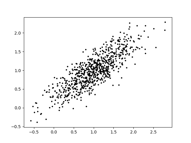
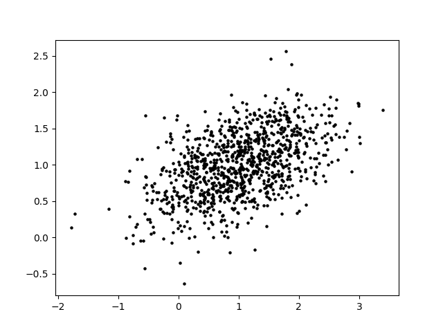
Now we’ll look at a simple example of PCA. Suppose you have a 2-variable scatterplot that you want to convert to a single-variable histogram. The first step is to identify a line that is the primary axis along which the data is arranged. The secondary axis, then, is a line perpendicular to this first line. We can find these axes using some matrix math, which I will omit here.

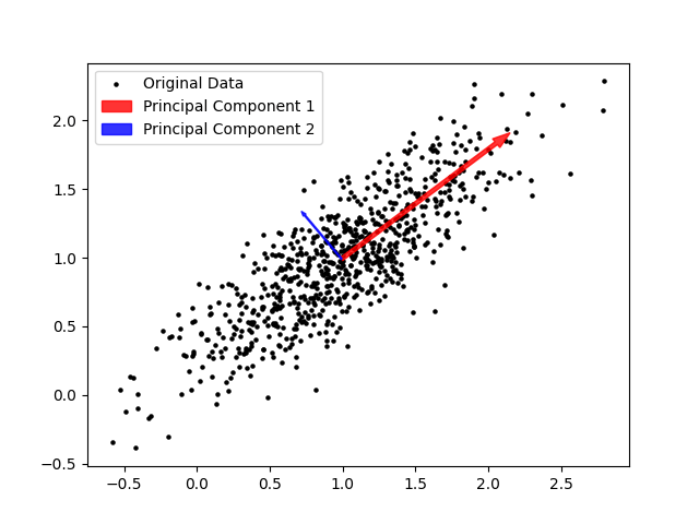
The principal components of the data set are a pair of vectors whose directions are defined by these axes and whose magnitudes are defined by the spread of the data set. A pair of perpendicular vectors like this creates what’s called a basis for 2D space, meaning we can use a change-of-coordinates formula to redefine the x and y axes. This is useful because it can make the data easier to work with. However, we can also simplify the data by “squishing it” along one axis. We no longer have that information about the data, but most of the information about the data is preserved and we now have a single axis along which the datapoints are arranged.

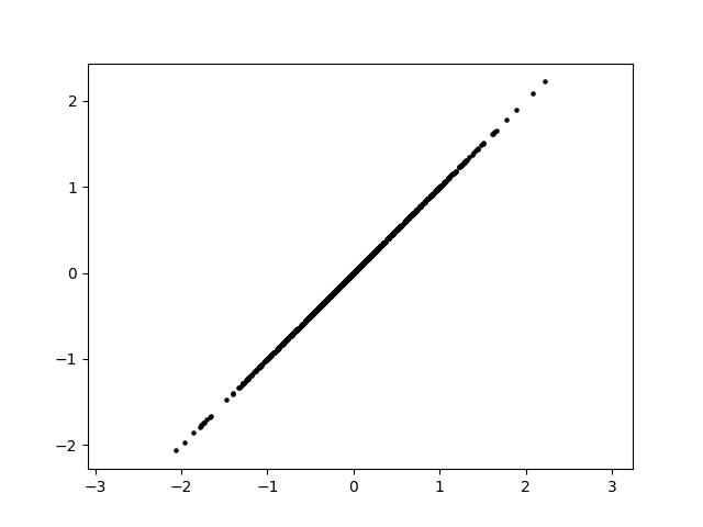
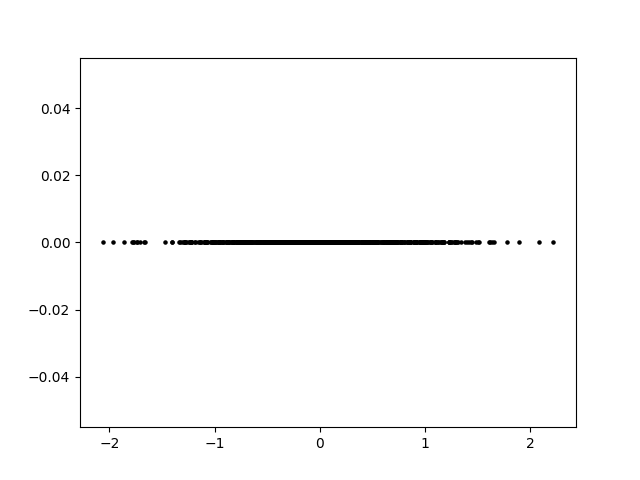
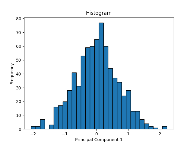
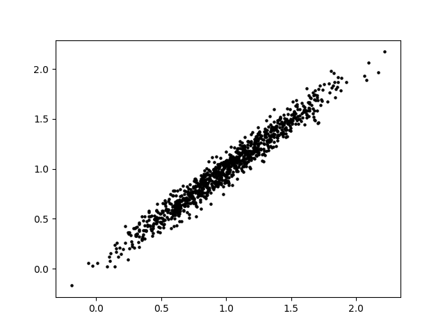
This strategy has a few useful applications. In statistics, it can be used to identify important relationships within the data and to investigate components separately. In AI applications, it is often used to reduce the total number of dimensions involved in order to speed up calculation. This is because the AI’s data could easily have hundreds of dimensions. Even by taking 100 dimensions down to 90, computation time will be saved. Depending on the situation, it may be easier or harder to reduce dimensions. In the example we looked at, most of the information about the data’s distribution is captured in principal component 1. However, it’s possible that neither principal component dominates, and reducing the dimension could therefore remove up to half of the information contained in our data set. Conversely, it’s possible for the data to be almost completely linear to begin with, such that reducing the dimension removes virtually no information. Additionally, depending on the application it may be more or less acceptable to lose information.

Summary

We looked at AI that use neural nets, which consist of an input, several “hidden” layers of neurons, and an output. The inputs and outputs are tensors, which are multidimensional arrays of numbers. From layer to layer of neurons, successive linear combinations (weighted sums) are calculated. The connection weights are determined by machine learning (training). This requires a preselected set of training data. To enhance the AI’s capabilities, the neural net architecture may include neurons that apply nonlinear functions or propagate information backwards. Since this type of AI entails a huge number of simple calculations, it is computationally difficult for an 8-core CPU, but relatively easy for a 1,000-core GPU. It is still considerably difficult, and computational complexity continues to be one of the barriers to smarter AI. There are many strategies for addressing this, including fine-tuning GPUs for tensor calculations, creating more efficient neural net architectures, as well as mathematical manipulation like using PCA to reduce dimensions.